Sampling Secrets -- How Statisticians Find the Truth

We live in an age of big data. Millions of data is collected by the second all over; weather data, shared posts and likes on social media, location data on our phones, credit card transactions, etc. Storing and analyzing this data requires a lot of expensive hardware, and so it is often useful to use only a portion of the data to perform quick analysis, and then extrapolating the results to the entire population. Sampling methods are essential techniques that allow researchers to study a subset of a population and make inferences about the whole. A strong sampling strategy leads to more accurate, reliable results. Sampling plans on the other hand, provide the statistical framework to measure the properties of a chosen sample in accordance with a specific goal. I will discuss both in this blog post.

📚 Table of Contents

1. Motivating Problem
2. Why Sampling?
3. Types of Sampling Methods
4. Sampling Plans
- 4.1 Solving the Motivating Problem – How Big Should Your Sample Be?
- 4.2 Building Machinery for Sampling Plans

1. Motivating Problem 🎯

Imagine you receive a delivery of 200 medical equipment , and that 10 of them are defective. You need to sample randomly from the batch to inspect for defects.
A natural question arises: How large should your sample be to have a high probability (say, 90 or 95%) of finding at least one defective item?

One might reasonably ask, “why not inspect all the equipment in order to be certain?” This may not be feasible when the inspection or testing process is resource or labor intensive. For instance, they may be a supply of vacutainers (used for blood work) that need to be tested for contamination or leakage. You could test all, but then you’ll have no equipment to use since they would have all been used in some way. This is because the tests is be distructive, so testing everything would defeat the purpose.

We would therefor explore a more elegant solution to this problem using 4. Sampling Plans after we have discussed the theory of sampling along with the motivation for choosing them them.

2. Why Sampling?

Sampling is the method of selecting a subset of a larger population. A sample is always with respect to a larger population, not necessarily the size.

For instance, selecting all 11 players of a soccer team for a study about that team is not a sample, since everyone in the team was used. When populations are too large to study entirely, sampling offer a practical solution. Instead of gathering data from everyone, we study a representative subset to save time, cost, and effort — while still drawing meaningful conclusions. The goal of sampling is to extrapolate the results to the entire population. Therefore, the way it is done is very important. If litte Johnny asks his 3 other friends their opinion of the little league baseball coach, it is a valid sample, but not a very representative the entire team’s opinion of the coach.

“Good sampling makes reliable statistics.”

Sampling is important because;

It is cost-efficient and less time consuming.
It is particularly useful when performing destructive experiments (say, performing crash tests of a new car model).
It is useful when working with and indeterminate or infinite population.

A sampling illustration.

3. Types of Sampling Methods

In Statistics, sampling methods refer to how we select a subset of a pupulation. There are many different ways to select a sample depending on the objective of the researcher. Researchers commonly use simple random sampling, but this is not always the ideal approach, depending on the application. Sampling methods fall into two major categories: Probability Sampling and Non-Probability Sampling.

3.1 Probability Sampling 🎲

Probability sampling ensures each individual has a known (and often equal) chance of selection, making it statistically sound.

Simple Random Sampling: 🎟️

Each element may be assigned a random number, and then using a random number generator, we may select a sample from the population based on the random numbers generated. The random number may be selected using any probability distribution function, although a uniform distribution is the most common choice.

Using a uniform distribution, each member of the population has a known equal chance of being selected (unless repetitions exist).
📌 Example 1: Picking names from a hat.

An illustration of simple random sampling .

Stratified Sampling: 🏛️

A population is divided into subgroups (strata) and a simple random sample is selected from each subgroup.
📌 Example: Sampling students from different academic majors.

A graphical representation of stratified sampling .

Cluster Sampling: 🏘️

A population is split into clusters, then entire clusters are randomly selected. This is similar to stratified sampling, except that we select entire subgroups, not individual elements from the subgroups. Each element in the population has a known equal probability of being selected. 📌 Example: Surveying a few randomly selected neighborhoods in a city as part of a study.

Systematic Sampling: 📏

Pick every k-th element from a list, starting from a random point. Systematic sampling is a form of simple random sampling. The selection of k is random, making each element equally likely to be selectted. Additionally, the units in the poplulation must be ordered for this to be feasible. 📌 Example: Surveying every 10th visitor to a museum.

3.2 Non-Probability Sampling 🔍

Non-probability sampling does not guarantee every individual an equal chance. It is often quicker and cost effective, but can be biased.

Convenience Sampling: ☕

This method involves sampling from whoever is easiest to reach.
📌 Example: Asking nearby shoppers for feedback.

Judgmental (Purposive) Sampling: 🧠

Selecting sample based on the researcher’s expert judgment.
📌 Example: Interviewing industry experts only.

Snowball Sampling: ❄️

Existing participants help recruit others.
📌 Example: Finding study subjects through referrals in niche communities.

Quota Sampling: 📊

Sampling specifically to meet predetermined characteristic quotas irrespective of how that characteristic is distributed in the population.
📌 Example: sample size of 20 to be made up of 40% men, 60% women in a survey for a population of 100 men and 30 women. This may be needed for a specific application. For instance, testing for an infection that is prevalent in women.

Within quota sampling, the underlying sampling method may be a simple random sample.

3.3 Choosing the Right Method

Choosing the right sampling method depends on:

Factor	Consideration
Research Objective	Accuracy vs. speed? Generalization needed?
Population Structure	Homogeneous or diverse?
Resources	Budget, manpower, time?
Bias Tolerance	Is some bias acceptable for faster results?

3.4 Example

Imagine you are a public health official tasked with estimating the average number of hours people exercise per week in a city of 500,000 residents.

😵 Interviewing every person is nearly impossible.
How can you efficiently gather accurate, representative data without surveying everyone?

➡️ Chosen Sampling Method: Cluster Sampling 🏘️

Why?

The city is geographically large.
Residents naturally live in neighborhoods (clusters).
It’s more practical to randomly choose a few neighborhoods and survey everyone in those neighborhoods.

📋 Steps:

Divide the city into 1,000 neighborhoods.
Randomly select 10 neighborhoods.
Survey all residents within the selected neighborhoods about their weekly exercise habits.
Analyze the collected data to estimate the city-wide average.

Conclusion

Sampling is both an art and a science.
The right technique ensures your data truly reflects your population, allowing confident, defensible decisions.

🔔 Takeaway:

“A well-designed sample can tell the story of a thousand data points — and sometimes, it’s all you need.” ✅ Tip: Most studies often employ a combination of probability sampling and non-probability sampling methods for research. —

4. Sampling Plans

Let us now consider the motivating problem;

We will use a probabilistic formulation to solve this problem. Then after building more machinery, we will revisit it once more.

Understanding the Problem

Total items: 200
Defective items: 10
Goal: Find the minimum sample size $n$ needed so that the probability of detecting at least one defective is x% or higher.

4.1 Solving the Motivating Problem – How Big Should Your Sample Be?

Each unit you draw has one of two outcomes; defective or not defective. So we have a binomial distribution.

Therefore the probability $p$ of selecting a defective item in one draw $P\text{(defective)} = \frac{\text{number of defectives}}{\text{total items}}= \frac{10}{200} = 0.05 = p$.

And the probability that a selected item is not defective, $q = 1- p = 1 - P\text{(defective)} = 0.95$

A choice of sample of size $n$, yields expected number of defectives, $E(\text{defectives}) = np$, with a standard deviation of $\sqrt{npq}$.

That is, by the central limit theorem, a sample of size $n=20$ is expected to contain:

$np \pm \;\sqrt{npq} = 20(0.05) \pm \;\sqrt{20(0.05)(0.95)} = [0,2)$ 65% of the time.
$np \pm 2\sqrt{npq} = 20(0.05) \pm 2\sqrt{20(0.05)(0.95)} = [0,3)$ 95% of the time.
$np \pm 3\sqrt{npq} = 20(0.05) \pm 2\sqrt{20(0.05)(0.95)} = [0,4)$ 99.7% of the time.

Result 1:
✅ Thus 95% of the time, we expect a simple randomly sample of size 20 to contain at most 3 defectives.

While this reasoning is robust, and quantifies the choice of sample size, we can do better. When can we guarantee the detection of a defective item if one exists? What about the probabilities? can we have more control over the level of confidence we desire to achieve?

If we draw $n$ items randomly, the probability that none of them is defective: $P\text{(no defectives)} = \left( \frac{190}{200} \right)^n$.

This implies that, the probability of finding at least one defective, $P\text{(at least one defective)} = 1 - \left( \frac{190}{200} \right)^n.$

Suppose we desire : $P\text{(at least one defective)} \geq x$. That is, $1 - \left( \frac{190}{200} \right)^n \geq x$.

Rearranging the inequality gives $\left( \frac{190}{200} \right)^n \leq 1 - x$.

Taking the natural logarithm on both sides: $n \geq \frac{\ln(1 - x)}{\ln\left( \frac{190}{200} \right)}$

A bar chart representation of sample size with corresponding probability of drawing at least one defective item. The graph shows that we need a ramdom sample size of 45 to guarantee a 90% chance of drawing a defective item.

Suppose you want a 95% chance of detecting at least one defective. Then $x = 0.95$, and: $n \geq \frac{\ln(1 - 0.95)}{\ln\left( \frac{190}{200} \right)}$

Using a calculator: $\ln(0.05) \approx -2.9957$ and $\ln(0.95) \approx -0.05129$

Thus:

\[n \geq \frac{-2.9957}{-0.05129} \approx 58.4\]

Result 2:
✅ You should sample at least 59 items to have a 95% chance of detecting a defective item. Not bad, but maybe we can use more intution of probability to set the boundaries of our confidence to provide more insight of this activity. We will visit that in the next section.

Please note that this does not contradict result 1. In the first result, we showed that a 95% of the time, a sample of size 20 will contain at most 3 defective (upper bound), but this does not guarantee existence. In order to guarantee existence, we will need to show that the lower bound is at least 1. In the first result, the lower bound was negative 1 (we round up to 0 when since we are analysing physical items).

To achieve an $x\%$ probability of finding at least one defective in a batch, we need a sample size, $n \geq \frac{\ln(1 - x)}{\ln\left( \frac{195}{200} \right)}.$

4.2 Building Machinery for Sampling Plans 🛠️

The goal of the remainder of this blog post is to help the reader:

Understand AQL, LTPD, and other components of sampling plans
Interpret OC curves
Generate sampling plans based on your needs

Consider this scenario, you are a manager of a juice plant and you receive 100 cubic yard containers of apples. You’ll want to check and make sure that all the apples in each container are good but you definitely cannot check every apple! Besides, taking a bite of each apple will leave it unfit for use (safety standards). You decide that a “bad” apple is one with a rotten spot so for inspection an apple is either “good” or “bad”. If there was one bad apple per container, would you return all the containers? No! If this were the case, you would be returning every container back to the seller so realistically it is okay to have a few bad apples There are about 1000 apples per container. You decide that:

If 10 apples (1%) are bad, this would be fine
If 50 apples (5%) are bad, you don’t want the container

A sampling plan quantifies risk and confidence:

How unlikely it is to get 10/1000 bad if the true defective rate is 10/1000?
How likely it is to get only 50/100 bad if the rate is 10/1000?

Acceptance Sampling applies to a specific lot.

You accept or reject that lot. It typically does not estimate the quality.

How many apples do you look at in each container before deciding you can accept it? If you look at all the apples this will take forever. Moreover, if the quality of the container is very bad, you will notice right away If the apples are very good, you will be inspecting forever. It will likely take a lot of selections to get to a bad apple.

In short, 100% inspection will not work. At some point you need to make a decision. A better way is to use a statistically based sampling plan. But, first some things to think about and understand.

In this figure, there are only 5 apples in a lot or container (1st column) with one bad apple(3). You are selecting two for inspection. There are 5 combination 2 ways (10 ways) of selecting two apples (columns 2 & 3: all possible 2 apple pair choices from the container). Since you are only choosing two, 4 out of 10 of the possible sample combinations show a 50% rate for “bad” apples.

Suppose we have a lot size of 5 and we select 2 apples. The probability of accepting the container is 60% since only 6 out of the 10 samples are entirely “good” (6 of 10 pairs good). The probability of rejecting the lot is 40% since 4 out of the 10 samples had “bad” units (4 of 10 pairs bad). This measures risk certainty; Repeated sampling would lead to rejecting the lot 40% of the time. For our lot of 1000 apples per pallet, the complexity increases significantly. Ts a result, it is at no surprise that the population and sample size affect our decision to accept or reject the lot.

You could be fortunate and select all of the bad apples thereby rejecting the delivery.

Alternatively, you could be fortunate and select all good apples thereby accepting the delivery.

The same principles/mathematics would apply to the motivation problem.

This scheme used to pass/fail (attributes) data is called Attributes Sampling Plans.

Attributes Sampling Plans are;

Tools used to quantify number of defective units in a batch: Use a small sample from a large batch to estimate the quality of the large batch. Pass the large batch if its estimated quality is good, otherwise fail it.
Used to quantify risk & certainty: Probability that a batch with many defective units will be detected. Probability that a batch with tolerably few defective units will pass.

Applications:

Incoming and outgoing quality inspection
Auditing files
Destructive testing

Useful Definitions

Defective Rate: The rate of units in a lot with non-conformities or differences distinguishing them from desirable units. Does not have to be actual defects.
Acceptable Quality Level (AQL): The maximum defect rate that is acceptable in a lot.
Alpha (): Probability of failing a good lot that meets AQL. Also known as producer’s risk, false alarm rate, or Type I error.
Lot Tolerance Percent Defective (LTPD): The minimum defect rate that should be rejected in a lot. Also known as Rejectable Quality Level (RQL). Note: LTPD must be higher than AQL The LTPD determines the protection provided by the sampling plan (Consumer error) not the AQL.
Beta (): Probability of passing a bad lot that exceeds LTPD. Also known as consumer’s risk, undetected problem rate, or Type II error.
Lot Size (N): The number of units in a large batch. Defect rate = (# of defective units in lot) / (lot size N)
Sample Size (n): The number of samples that will be taken from the lot, . We estimate the lot defect rate using the sample defect rate
Lot Tolerance Percent Defective (LTPD): The minimum defect rate that should be rejected in a lot. Also known as Rejectable Quality Level (RQL).
- LTPD must be higher than AQL.
- The LTPD determines the protection provided by the sampling plan (Consumer error) not the AQL.
Acceptance Number (c): The maximum number of defective units in a sample (n) that you can find and still pass the sampling plan Ensures rate of AQL will pass % of time and rate of LTPD fails % of time usually determined by software.
P control chart (Percent control chart ) or ImR control chart – .
If n is very large hundreds to thousands use ImR control chart.
Used to track trends in data. Makes Acceptance sampling more effective.
Overall average fraction non-conforming can provide an approximate idea of Supplier Quality Level. Control Limits provide us with a sense of how variable product quality is.

Check a Normal Probability Plot / Quantile Plot Assumes the data are bell shaped (Normal Distribution).

S control chart or mR control chart Used to track trends in data. Makes acceptance variables sampling more effective.
Standard deviation tracked Control Limits provide us with a sense of how variable product quality is. Formulas for variables sampling rely on consistent lot variation.

Attribute Sampling Plans

In every sampling plan, the lot size, $N$, the sample size, $n$, and the number of conforming units $c$, are the most important. If you sample $n$ units from of a lot of $N$ and only pass the lot if you find no more than $c$ defective units:

The probability of finding exactly $d$ nonconforming units in a sample of size $n$ drawn without replacement from a lot of size $N$ containing $D$ nonconforming units is given by the Hypergeometric Distribution:
\[h(d; n, D, N) = \frac{\binom{D}{d} \binom{N - D}{n - d}}{\binom{N}{n}}\]
Where:
- $n$ = sample size
- $N$ = lot size
- $d$ = number of nonconforming units found in a sample of size $n$
- $D$ = number of nonconforming units in the lot of size $N$
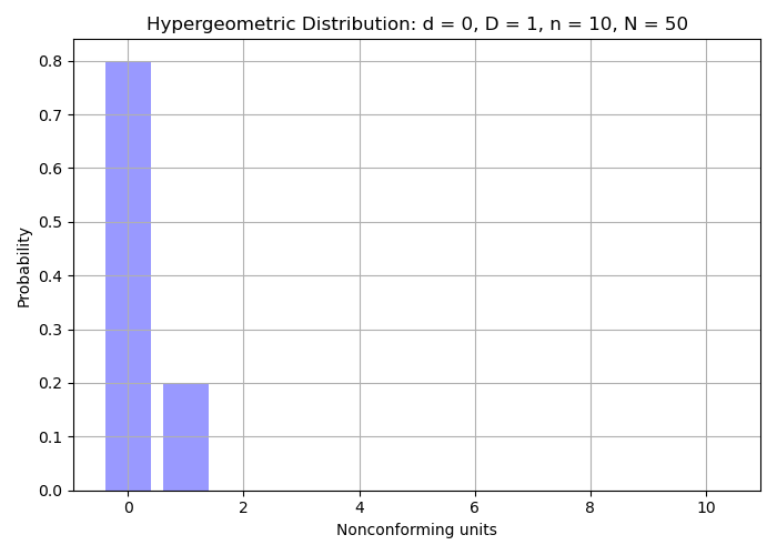
Example

Problem: What is the probability of accepting a lot with no nonconforming units detected (i.e., $d = 0$), using a sample size of $n = 10$, when the process nonconforming rate is 2%?
- $d = 0$,
- $D = 1$ (since $50 \times 0.02 = 1$),
- $n = 10$,
- and $N = 50$
Then:
\[H(0; 10, 1, 50) = \frac{\binom{1}{0} \binom{49}{10}}{\binom{50}{10}} \approx 0.800\]
Interpretation:
Using a sample size of $n = 10$ and accepting only if $d = 0$ (i.e., no defects found), there is an 80% chance of accepting a process with 2% nonconforming rate.
- The binomial coefficient $\binom{a}{b}$ is defined using factorials:
\[\binom{a}{b} = \frac{a!}{b!(a - b)!}\]
- For example:
  $50! = 50 \times 49 \times 48 \times \cdots \times 1$ Factorials grow rapidly, which is why software tools or approximations are often used for computations.
Probability distribution of accepting a lot with for a number of nonconforming units detected.
The Binomial Distribution gives the probability of finding exactly $d$ nonconforming units in a random sample of size $n$ when the probability of a nonconforming unit on any single draw is $p$. The probability mass function is;
\[b(d; n, p) = \binom{n}{d} p^d (1 - p)^{n - d}\]
where,
- $n$: sample size
- $d$: number of nonconforming units found in a sample of size $n$
- $p$: probability of a nonconforming unit on a single draw
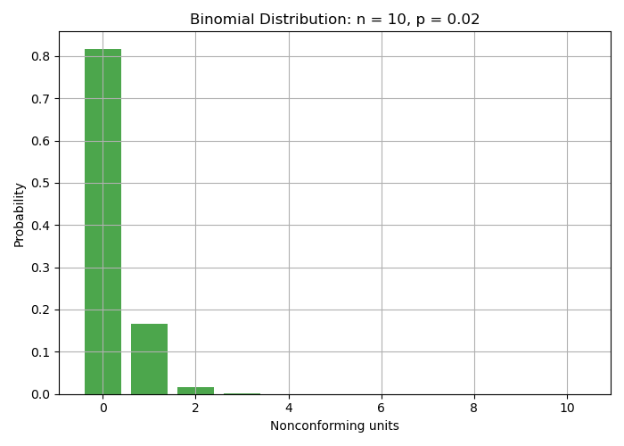
Example

Suppose a process has a nonconforming rate of $p = 0.02$ (2%). We take a sample of size $n = 10$, and we want the probability of finding zero nonconforming units in the sample.
- $n = 10$
- $d = 0$
- $p = 0.02$
We compute:
\[b(0; 10, 0.02) = \binom{10}{0}(0.02)^0 (1 - 0.02)^{10} = (1)(1)(0.98)^{10} \approx 0.817\]
Thus, using a sample size of $n = 10$ and accepting only if $d = 0$, we have approximately an 81.7% chance of accepting a process with a 2% nonconformance rate under the binomial approximation.

The binomial distribution is an approximation to the hypergeometric distribution. A rule of thumb for using the binomial approximation is when:
\[\frac{n}{N} \leq 0.10\]
That is, the sample size is no more than 10% of the population size, so sampling without replacement behaves approximately like sampling with replacement.

Probability distribution of accepting a lot with for a number of nonconforming units detected
The Poisson distribution models the probability of a given number of events occurring in a fixed interval or space, assuming the events happen independently and the average rate is constant.

The probability mass function is:
\[P(d; \lambda) = \frac{e^{-\lambda} \lambda^d}{d!}\]
Where:
- $d$ = number of occurrences of nonconforming units in the sample
- $\lambda$ = expected number of nonconforming units in the sample
- and $e\approx 2.7183$.
The Poisson distribution is also a good approximation to the binomial distribution when:
\[\frac{n}{N} \leq 0.10 \quad \text{and} \quad p \leq 0.10\]

Example

Continuing the example from the hypergeometric and binomial cases:
- $N = 50$ (lot size)
- $n = 10$ (sample size)
- $p = 0.02$ (nonconforming rate)
- and $\lambda = np = 10 \times 0.02 = 0.2$
Probability of 0 nonconforming units:
\[P(0; 0.2) = \frac{e^{-0.2} \cdot 0.2^0}{0!} = e^{-0.2} = 0.8187\]
Probability of 1 nonconforming unit:
\[P(1; 0.2) = \frac{e^{-0.2} \cdot 0.2^1}{1!} = 0.8187 \times 0.2 = 0.1637\]
Total probability of accepting the lot (0 or 1 nonconforming):
\[P(0 \text{ or } 1) = 0.8187 + 0.1637 = 0.9824\]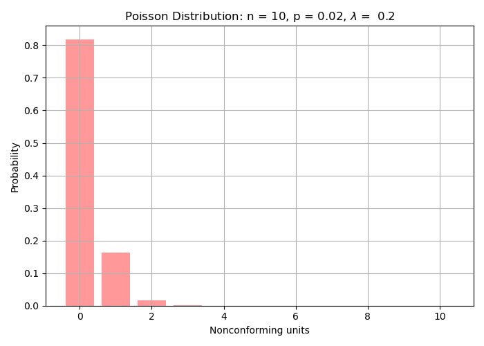

Probability distribution of accepting a lot with for a number of nonconforming units detected
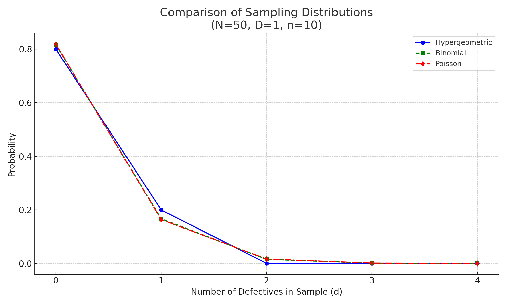
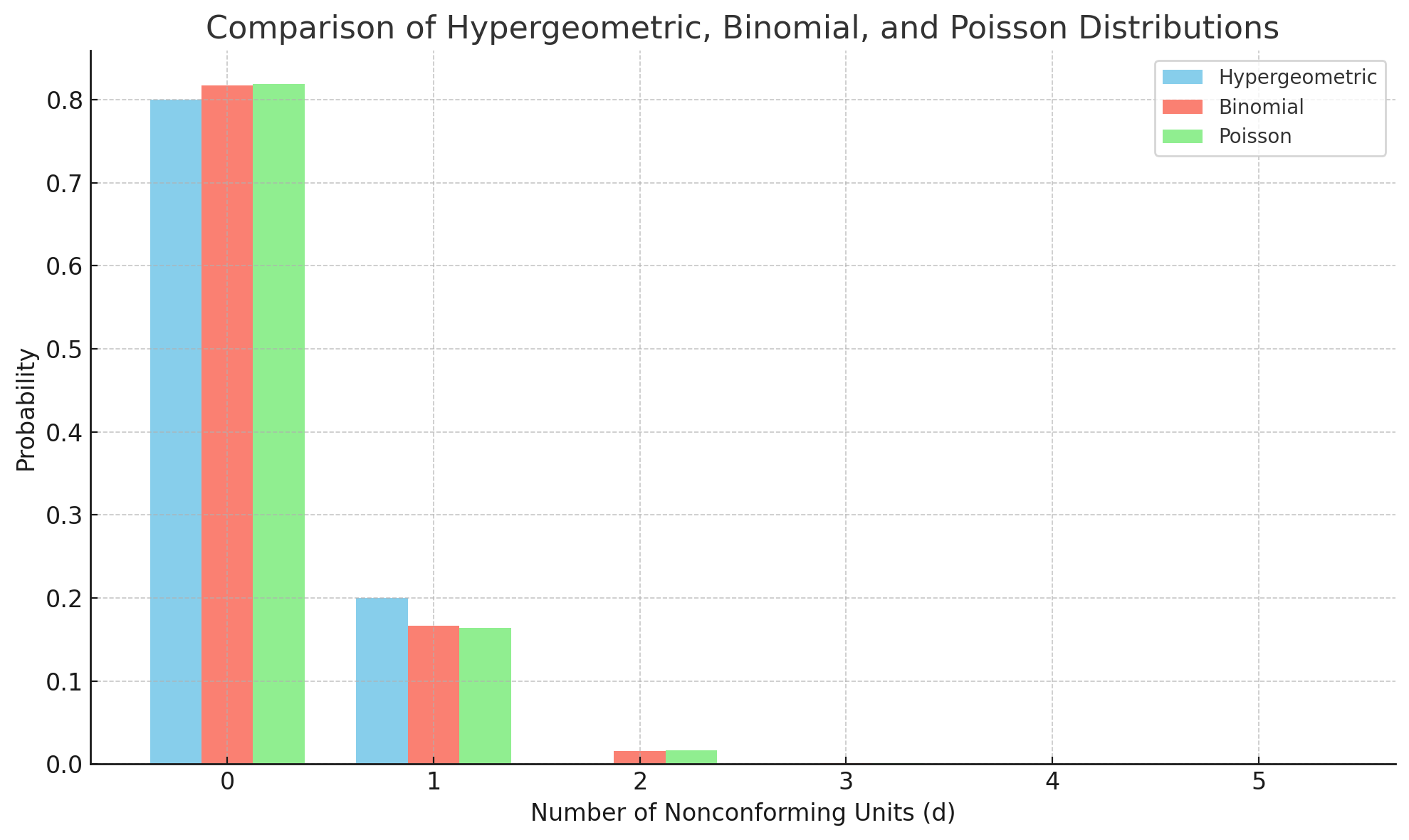Comparing Hypergeometric, Binomial, and Poisson Distributions. Probability distribution of accepting a lot with for a number of nonconforming units detected

The risk associated with a sampling plan can be read from the operating characteristic (OC) curve. The OC curve is a graph which shows the probability, $P_a$ of a lot acceptance for different lot quality levels.

Given a sampling plan $(N, n, c)$, and the lot quality level $p$, the lot acceptance can be calulated using;

$P_a = P(X\leq c) = \sum_{i=0}^{c} \frac{\begin{pmatrix}Np\\ i\end{pmatrix} \begin{pmatrix}N - Np\\ n - i\end{pmatrix}}{\begin{pmatrix}N\\ n\end{pmatrix}}, c=0, 1,2,\ldots,\min(n, Np)$, Np should be an integer or rounded.
Alternatively, $P_a = P(X\leq c) = \sum_{i=0}^{c} \begin{pmatrix}n\\ i\end{pmatrix} p^i (1-p)^{n-i}$

For the actual lot sampling, a systematic sample is often the best since items may be stacked in boxes. Say, select every 12th item. This reduces the temptation for convinient sampling. A random number may be used, although $\frac{\text{sample size}}{\text{lot size}}$ can provide an unbiased number.

Other probabilistic samples too may be chosen. Although the samples in the batch should be independent, and the lot size $N$ should be large (at least 10 times greater than the calculated sample size $n$).

Operating Characteristic (OC) Curves:

The probability of passing an attributes plan against possible defect rates in the lot.

X-axis: hypothesized lot defective rate

Y-axis: probability of c or fewer defective units in a sample of n from a lot of N given lot defective rate.

There are two kinds of OC curves. Type A assumes finite lot size and uses the hypergeometric distribution. Type B assumes infinite lot size. ($N > 10\times n$, where N= lot size, n = sample size.) Use Binomial or Poisson.

If you sample n units from of a lot of N and only pass the lot if you find no more than c defective units: You can be certain that lots with AQL defect rate will pass You can be certain that lots with LTPD defect rate will fail If the lot passes, you are certain that the defect rate is no more than LTPD If a lot fails, you are not sufficiently certain that it meets LTPD. Do not keep sampling until a sample passes – this forces Type II Error (undetected problems)! However, do complete the sample so that we can get a good estimate of the defect rate.

Long-term statistics are assumed. (Grant p406)

Given a statistically controlled process that has a fraction non-conforming . The following is true: Each random sample of size n selected from a lot of N items will essentially be a random sample from the process that has the fraction non-conforming . Type A OC curves are based on the hypergeometric distribution. A type B OC curve will provide the expected results of the sampling plan. Based on either Binomial or Poisson. Most people use Type B OC curves.

In different words, If a process is statistically in-control the OC curve will provide the expected $P_a$ given Lot Percent Defective. In the real world, this is not always true.
Suppliers do not always ship product from processes that are in-stat control…. Therefore, the OC curve Pa will be approximate.
It however, does provide guidance.

Note: Random sample is another term for in-statistical control.