Equivalence Concordance Rate (ECR): Calibrating Equivalence Acceptance Criteria
How do you know whether a chosen equivalence margin is actually a good one? The Equivalence Concordance Rate (ECR) framework answers that question — not by proposing yet another margin, but by measuring how coherently any proposed margin makes decisions.
When a pharmaceutical process changes — a site transfer, a scale-up, a new piece of equipment — regulators expect evidence that the product is comparable before and after. The standard tool is the Two One-Sided Tests (TOST) procedure, and the whole verdict hangs on a single pre-specified number: the Equivalence Acceptance Criterion (EAC), the margin \(\Delta\) within which two process means count as “the same.”
Set it too wide and a shifted process is wrongly accepted; too narrow and an acceptable process is wrongly rejected. Many recipes for setting the margin coexist — \(\sigma\)-scaled, percent-of-mean, effect-size, capability-linked — but they are seldom ranked by the coherence of the decisions they induce. ICH Q5E deliberately specifies no single statistical method, which leaves the choice to the analyst without a common yardstick.
The goal of this work. Not a new hypothesis test, and not a new margin. A calibration and comparison framework that takes any candidate EAC — however derived — and scores how well it supports coherent decisions, so competing margins can be ranked and tuned on a level playing field.
Because the diagnostic sweeps hypothetical shifts around an estimated process, a single comparability dataset is enough to benchmark whatever margin you are currently using.
The idea: score a margin by whether two tests agree
Apply two tests to the same before/after dataset:
- a difference test (D-test), a two-sided \(t\)-test asking “is there any detectable difference?”, and
- an equivalence test (E-test), TOST against \(\pm\Delta\), asking “is the shift small enough to be practically irrelevant?”
A well-calibrated margin makes these two verdicts agree. Crossing their outcomes gives four zones:
| E-test pass (equivalence concluded) | E-test fail (equivalence not concluded) | |
|---|---|---|
| D-test fail (no difference) | Z₁ ✓ Concordant-equivalent | Z₂ ? Gray zone |
| D-test pass (difference) | Z₃ ! Paradox | Z₄ ✓ Concordant-different |
Estimating the zone frequencies by Monte Carlo at each true shift gives three curves that sum to 1:
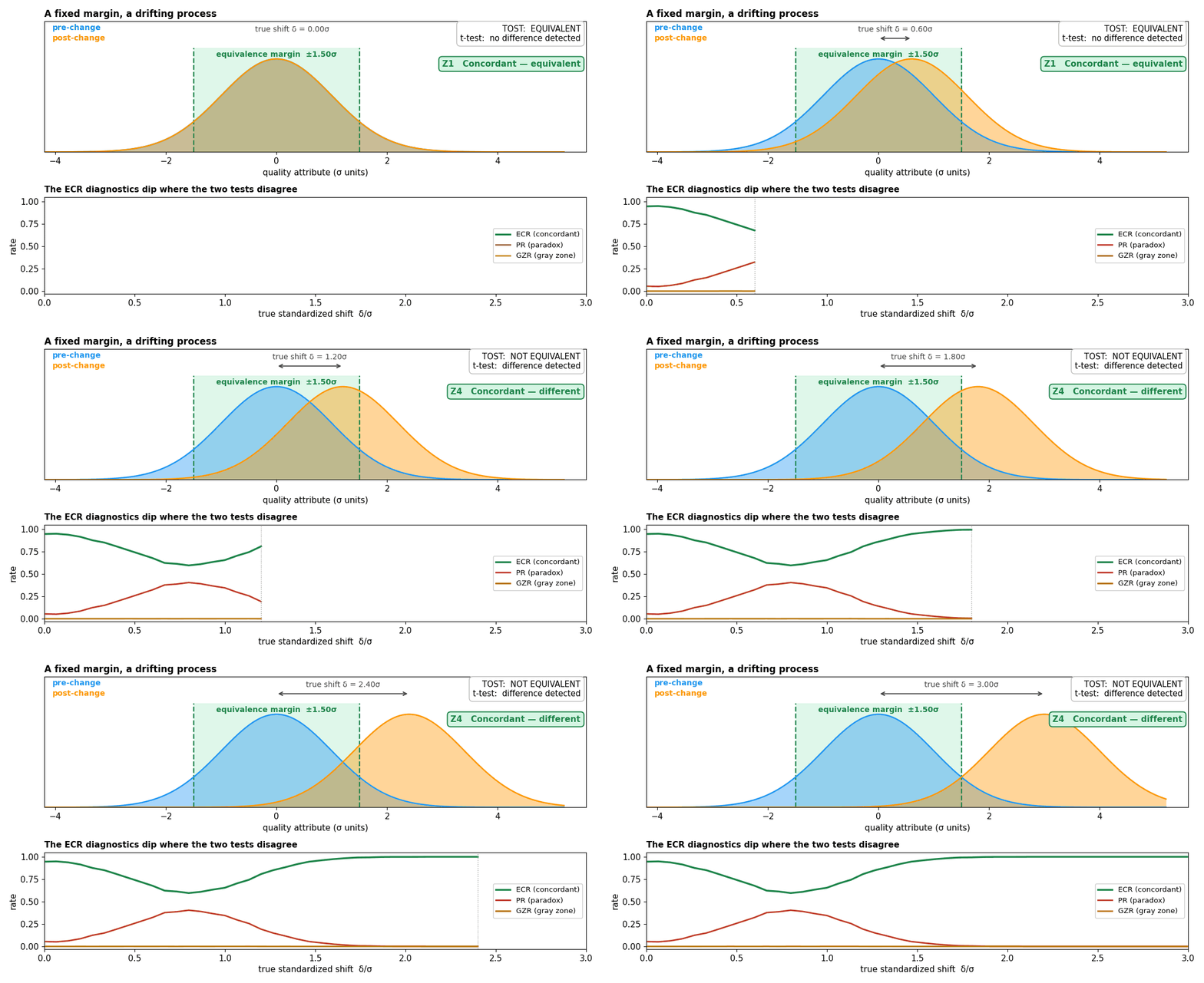
\[ECR = \frac{Z_1 + Z_4}{N},\qquad PR = \frac{Z_3}{N},\qquad GZR = \frac{Z_2}{N}.\]High ECR means coherent decisions; high PR means the margin is wide relative to detectability; high GZR means it is too narrow or the study is underpowered. Averaging the ECR curve over the shift range collapses it to one rankable scalar, the integrated ECR:
\[iECR = \frac{1}{u_{max}} \int_0^{u_{max}} ECR(u)\, du, \qquad u = \delta/\sigma_{pre}.\]Two clarifications matter. First, PR is not a false-acceptance rate — because the D-test has a point null and flags any detectable shift, a paradox can arise even when TOST correctly declares equivalence for a shift genuinely inside the margin. PR measures disagreement, not error. Second, the two disagreement modes are opposite directions of decision risk: a paradox is the consumer’s-risk direction, a gray zone the producer’s-risk direction. Reporting them separately lets a practitioner weigh both.
Seeing it move
The animation below holds the margin fixed at \(1.5\,\sigma\) and lets the post-change process drift. At small shifts both tests agree the process is fine. Past a point the \(t\)-test starts detecting a difference while TOST still concludes equivalence — the paradox zone — before the two finally agree again that the process has moved.
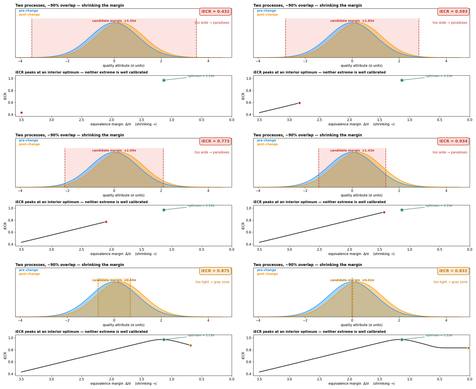
Now hold the shift fixed instead (two processes overlapping about 90%) and sweep the margin. A very wide margin waves through shifts the \(t\)-test can see; a margin near zero can never conclude equivalence at all. iECR peaks in between — and that interior optimum is exactly what the framework is built to locate.
The case study: four common margins
To demonstrate the framework end-to-end the paper scores four structurally distinct margins, each encoding a different philosophy of a tolerable shift. These are a case study, not a contribution — and the tuning values are illustrative rather than established standards. Only Method A’s \(\lambda\) has an external anchor (the FDA’s draft Tier-1 analytical-similarity criterion, withdrawn in 2018); C’s \(ES\) is matched to it, and B and D take round conventional values.
| Method | Formula | Anchored to | Default |
|---|---|---|---|
| A. \(\sigma\)-Scaled | \(\mathrm{EAC}_A = \lambda\,\sigma_{pre}\) | process variability | \(\lambda=1.5\) |
| B. Percent-of-Mean | \(\mathrm{EAC}_B = \lambda_\%\,\mu_{pre}\) | the mean level | \(\lambda_\%=0.05\) |
| C. Effect-Size | \(\mathrm{EAC}_C = ES\cdot\hat\sigma_{upper}\) | assumed effect size \(+\) a \(\chi^2\) variance correction | \(ES=1.5\) |
| D. Ppk-Informed | \(\mathrm{EAC}_D = \max(d_{pre}-3\,Ppk_{target}\,\sigma_{pre},\,0)\) | process capability and spec limits | \(Ppk_{target}=0.8\,Ppk_{pre}\) |
Two structural points carry most of the story later:
Method C is Method A plus a variance hedge. With \(c=\sqrt{(n_{pre}-1)/\chi^2_{\alpha,\,n_{pre}-1}}\ge 1\), \(\mathrm{EAC}_C = ES\cdot\sigma_{pre}\,c \to \lambda\,\sigma_{pre} = \mathrm{EAC}_A\) as \(n_{pre}\to\infty\). That inflation — about \(1.6\times\) at \(n_{pre}=10\) — is their only structural difference, making A-vs-C a clean controlled test of the correction itself.
The Ppk margin, generalized off-center. Real processes are never centred between their limits, so the paper replaces the spec half-width with \(d_{pre}\), the distance from the mean to the nearest limit. This closed form and its off-center derivation are contributions of the paper. It comes with a feasibility boundary: the margin vanishes once \(Ppk_{target}\ge Ppk_{pre}\), so anchoring to current capability collapses it to zero. Using a capability retention fraction \(\rho\in(0,1)\) with \(Ppk_{target}=\rho\,Ppk_{pre}\) gives the tidy \(\mathrm{EAC}_D = d_{pre}(1-\rho)\), which is always feasible.
The experiment
Because every test decision depends only on ratios, the study fixes \(\sigma_{pre}=1\) and varies six dimensionless drivers over a constrained factorial grid:
| Midpoint \(m/\sigma_{pre}\) | Spec \(S/\sigma_{pre}\) | Sample size \(n_{pre}\) | Ratio \(r=n_{post}/n_{pre}\) | SD ratio \(\sigma_{post}/\sigma_{pre}\) | Off-center \(\kappa\) | |
|---|---|---|---|---|---|---|
| Values | 5, 10, 15, 25, 35, 50 | 2.5, 5, 10 | 4, 8, 12, 16, 20, 24, 28, 30 | ⅓, ½, 1, 2 | 0.5, 0.75, 1.0, 1.25, 1.5, 2.0 | 0.05, 0.10, 0.20, 0.35 |
| Levels | 6 | 3 | 8 | 4 | 6 | 4 |
What the results say
Only the top of the ranking is stable
Averaged over the whole grid at prespecified defaults, the \(\sigma\)-scaled Method A is the most robust general-purpose choice — but the paper is careful about how much weight the rest of the ordering can bear.
| Method | mean iECR | SD | iPR (paradox) | max GZR (gray) |
|---|---|---|---|---|
| A. \(\sigma\)-Scaled | 0.872 | 0.107 | 0.036 | 0.220 |
| C. Effect-Size | 0.822 | 0.101 | 0.165 | 0.028 |
| D. Ppk-Informed | 0.808 | 0.112 | 0.020 | 0.596 |
| B. %-of-Mean | 0.800 | 0.112 | 0.054 | 0.501 |
Mean iECR spans only 0.800–0.872, and the lower three fall within 0.022 of one another — C and D differ by 0.014 and reverse under other scenario mixes. Per scenario, A is highest in 47% of the grid and lowest in only 2%, while B, C, and D are each lowest in 28–36%, so none of them is reliably the weakest. What is clear is the trade-off structure: C is the most paradox-prone, D the most gray-zone-prone.

Sample size dominates — and cuts both ways
A Type-II ANOVA puts sample size far ahead of everything else (\(\eta^2 = 0.290\), a large effect), followed by the method \(\times\) variance-ratio interaction (0.118) and method itself (0.066). That method choice is a substantive main effect is precisely what justifies a systematic comparison framework.

All methods improve steeply to \(n_{pre}\approx12\) — but then C turns over near 16 and A near 24, because the overpowered point-null \(t\)-test begins flagging trivially small shifts, widening the paradox window for the wider margins. More data is not uniformly better.
Unequal variance splits the methods. As the post-change spread inflates, A, B, and D decline while Method C alone improves, overtaking A beyond \(\sigma_{post}/\sigma_{pre}\approx1.5\): inflating the spread enlarges the standard error and pushes everything toward the gray zone, which harms tight margins but corrects C’s over-wide one. Repeating the analysis with Welch–Satterthwaite versions of both tests preserves the crossover, so this is genuine rather than an artifact of pooling.
Tuning does not make the methods converge
At their respective optima a \(\approx\)9-point iECR gap persists, so the differences are structural rather than artifacts of the defaults. Each optimum is also a broad plateau, not a sharp point — practically, a tuning constant only needs to land in the right neighbourhood.

| Method | Optimum | Peak iECR | Flat within 0.005 over |
|---|---|---|---|
| C. Effect-Size | \(ES^*=1.00\) | 0.930 | \([0.93,\,1.07]\) |
| A. \(\sigma\)-Scaled | \(\lambda^*=1.43\) | 0.908 | \([1.29,\,1.50]\) |
| D. Ppk-Informed | \(\rho^*=0.83\) | 0.842 | \([0.80,\,0.86]\) |
| B. %-of-Mean | \(\lambda_\%^*=0.039\) | 0.836 | \([0.030,\,0.044]\) |
The most interesting reversal. Tuned, Method C (0.930) overtakes Method A (0.908) — even though C’s optimal effect size sits below A’s coefficient. Since the two differ only by the \(\chi^2\) correction, this is direct evidence that the correction helps once calibrated. C’s poor showing at defaults is an artifact of naively matching \(ES\) to A’s \(\lambda=1.5\), which over-widens the realized margin and inflates paradoxes — not a flaw in the correction.
Choosing a margin in practice
The paper frames selection around scientific purpose rather than a numerical threshold. That purpose is what has to be defensible; everything else refines it.
First, what is the margin’s scientific basis?
- Capability preservation → Method D, with \(\rho\in[0.7,0.9]\).
- Variability scaling → Method A, with \(\lambda\in[1.0,1.5]\).
- Effect-size reasoning → Method C, with \(ES\approx1.0\).
Then adjust for:
- Unequal spread. If \(\sigma_{post}/\sigma_{pre}\gtrsim1.5\) is plausible, prefer C — the only method that improves under inflation.
- Small \(n_{pre}\). C’s \(\chi^2\) bound inflates its margin as \(n_{pre}\) shrinks; check the realized \(\mathrm{EAC}/\sigma_{pre}\).
- Capability feasibility. A relative target is always feasible; a fixed one requires \(d_{pre}/\sigma_{pre}>3\,Ppk_{target}\). If it fails, relax the target — don’t switch method, which sets the capability requirement aside rather than satisfying it.
- No dominant purpose. Default to A, whose prespecified \(\lambda=1.5\) already falls inside its optimal plateau.
Method B is deliberately absent. Its mean-scaled margin swings between paradox-prone at large \(m/\sigma\) and over-tight at small \(m/\sigma\); check what it actually implies at your own \(\mu_{pre}/\sigma_{pre}\) before adopting it.
One distinction the paper insists on: planning computes these curves before a confirmatory study to justify a margin that is then prespecified, whereas diagnostic benchmarking scores an incumbent margin against an observed process and is exploratory only — never grounds for retrospectively changing a pre-specified margin.
On real data
Applied to three attributes of a real bulk-versus-packaged comparability dataset, the diagnostic compares the ECR-recommended margin against an incumbent fixed \(3\,s_{pre}\) rule:
{
  "data": [
    {"x": ["Assay", "Impurities", "Water"],
     "y": [0.961, 0.971, 0.934],
     "name": "ECR-recommended margin",
     "type": "bar",
     "marker": {"color": "#2196F3"},
     "text": ["0.961<br>(Effect-Size)", "0.971<br>(Ppk-Informed)", "0.934<br>(σ-Scaled)"],
     "textposition": "outside"},
    {"x": ["Assay", "Impurities", "Water"],
     "y": [0.557, 0.977, 0.663],
     "name": "Incumbent 3·s_pre",
     "type": "bar",
     "marker": {"color": "#FF9800"},
     "text": ["0.557", "0.977", "0.663"],
     "textposition": "outside"}
  ],
  "layout": {
    "title": {"text": "iECR: recommended vs. incumbent margin on real comparability data", "font": {"size": 14}},
    "yaxis": {"title": "iECR", "range": [0, 1.15]},
    "barmode": "group",
    "legend": {"orientation": "h", "y": -0.15},
    "margin": {"t": 40, "b": 60},
    "font": {"size": 11}
  }
}
For assay and water the recommended margin is decisively better — the \(3\,s_{pre}\) rule is far too wide, driving its peak paradox rate to 0.990 and 0.811. For impurities the two are essentially tied (0.971 vs 0.977), and the choice then rests on which error matters more: the Ppk-informed margin gives the lower gray-zone rate, the incumbent the lower paradox rate. Surfacing that trade-off, rather than declaring a winner, is the point of the diagnostic.
Conclusion
The Equivalence Concordance Rate framework is a decision-quality lens for equivalence-margin specification — not a new test, and not a new margin. It separates wide-margin failure (paradox, consumer’s risk) from narrow-margin failure (gray zone, producer’s risk), collapses a margin’s full shift-response into one rankable score, and needs only pre-change data, so a single comparability dataset suffices to benchmark an incumbent margin.
Applied to four common margins across 10,368 scenarios — not to crown a single best margin — it finds the methods separate structurally rather than by tuning, with sample size the dominant driver. Below the top spot the ordering is close enough that it should not be over-read.
The takeaway for practitioners: rather than defending a margin by tradition, you can justify it with quantitative evidence — run a targeted ECR study and compare your candidate against the alternatives, for your own process and your own sample sizes.
Download
- Full paper PDF: Equivalence Concordance Rate (ECR) Framework
Enjoy Reading This Article?
Here are some more articles you might like to read next: